2. Histogram equalization
2.1. Histogram equalization
Image spatial domain processing is an important image processing technology. This type of method is directly based on the pixel operation of the image and is mainly divided into two categories: grayscale transformation and spatial domain filtering. Histogram equalization is a commonly used grayscale transformation method. Usually, the components of the dark image histogram are concentrated at the lower grayscale end, while the components of the bright image histogram tend to the higher grayscale end.
If the grayscale histogram of an image almost covers the entire grayscale value range, and except for the number of individual grayscale values that are more prominent, the entire grayscale value distribution is approximately uniform, then this image has a larger grayscale dynamic range and higher contrast, and the image details are richer. It has been proved that relying solely on the histogram information of the input image, a transformation function can be obtained, and the input image can achieve the above effect using this transformation function. This process is histogram equalization.
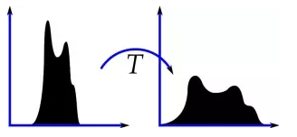
The left side of the picture is the histogram, and the right side is the histogram equalization effect.
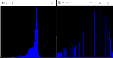
Histogram equalization is to stretch the original histogram so that it is evenly distributed in the entire grayscale range, thereby enhancing the contrast of the image.
The central idea of histogram equalization is to change the grayscale histogram of the original image from a relatively concentrated area to a uniform distribution in the entire grayscale range.
It aims to make the overall effect of the image uniform, and the points between each pixel level between black and white are more uniform.
Function: cv2.equalizeHist()
2.2 Actual effect display
Source code path:
/home/pi/DOGZILLA_Lite_class/4.Open Source CV/D.Image_Enhancement/02_Histogram_Equalization.ipynb
ximport cv2import numpy as npimport matplotlib.pyplot as pltimg = cv2.imread('yahboom.jpg',1)gray = cv2.cvtColor(img,cv2.COLOR_BGR2GRAY)#cv2.imshow('src',gray)dst = cv2.equalizeHist(gray)#cv2.imshow('dst',dst)#cv2.waitKey(0)gray = cv2.cvtColor(gray, cv2.COLOR_BGR2RGB)dst = cv2.cvtColor(dst, cv2.COLOR_BGR2RGB)#plt绘制前后两张图片显示效果 Display effect of two pictures before and after plt drawing#源图显示 Display source imageplt.figure(figsize=(14, 9), dpi=100)#设置绘图区域的大小和像素 Set the size and pixels of the drawing areaplt.subplot(121) # 一行两列第一个 The first one of two columnsplt.imshow(gray)#灰度 直方图均衡化 Grayscale Histogram Equalizationplt.subplot(122) # 一行两列第二个 The second one in one row and two columnsplt.imshow(dst)plt.show() 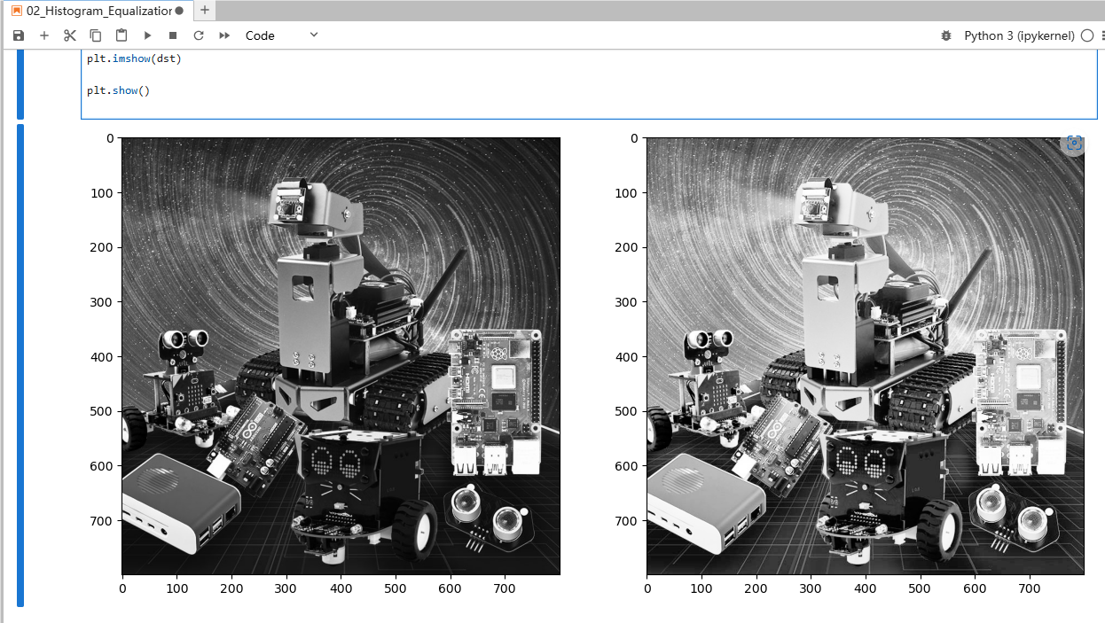
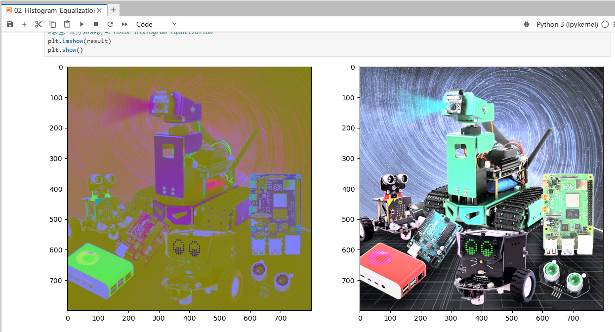
xxxxxxxxxximport cv2import numpy as npimg = cv2.imread('yahboom.jpg',1)# cv2.imshow('src',img)(b,g,r) = cv2.split(img)#通道分解 Channel decompositionbH = cv2.equalizeHist(b)gH = cv2.equalizeHist(g)rH = cv2.equalizeHist(r)result = cv2.merge((bH,gH,rH))# 通道合成 Channel synthesis# cv2.imshow('dst',result)# cv2.waitKey(0)img = cv2.cvtColor(img, cv2.COLOR_BGR2RGB)dst = cv2.cvtColor(dst, cv2.COLOR_BGR2RGB)#plt绘制前后两张图片显示效果plt.figure(figsize=(14, 9), dpi=100)#设置绘图区域的大小和像素 Set the size and pixels of the drawing areaplt.subplot(121) # 一行两列第一个 The first one of two columnsplt.imshow(img)plt.subplot(122) # 一行两列第二个 The second one in one row and two columns#彩色 直方图均衡化 Color Histogram Equalizationplt.imshow(dst)plt.show()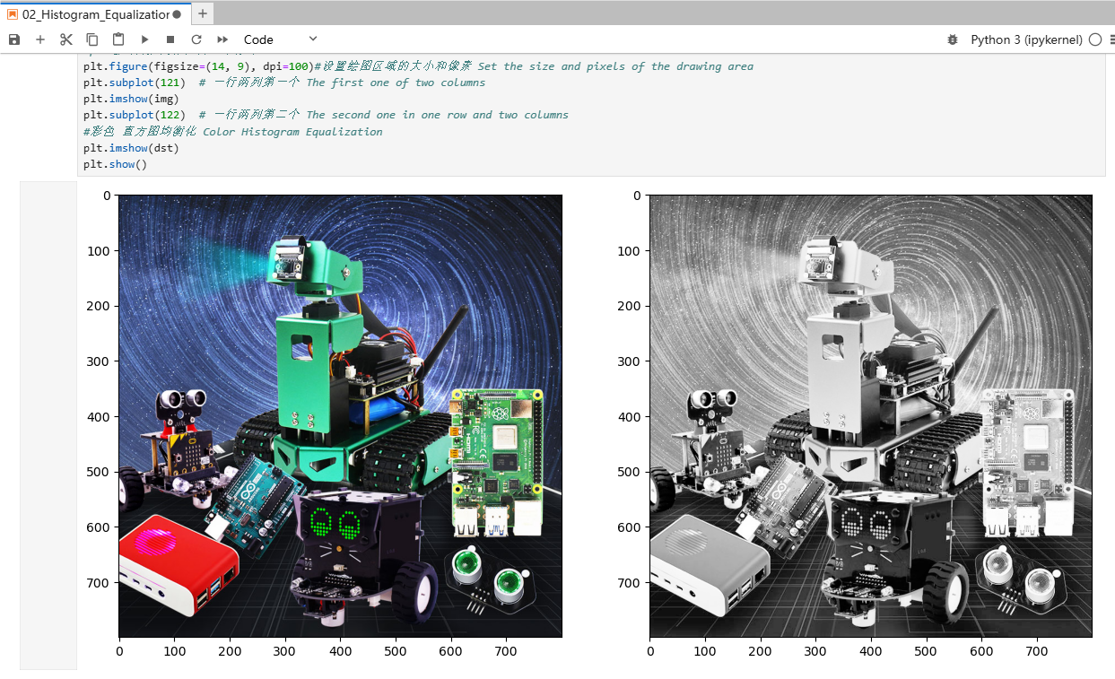
xxxxxxxxxximport cv2import numpy as npimg = cv2.imread('yahboom.jpg',1)imgYUV = cv2.cvtColor(img,cv2.COLOR_BGR2YCrCb)# cv2.imshow('src',img)channelYUV = cv2.split(imgYUV)ggg = list(channelYUV)ggg[0] = cv2.equalizeHist(channelYUV[0])channelYUV = tuple(ggg)channels = cv2.merge(channelYUV)result = cv2.cvtColor(channels,cv2.COLOR_YCrCb2BGR)# cv2.imshow('dst',result)# cv2.waitKey(0)imgYUV = cv2.cvtColor(imgYUV, cv2.COLOR_BGR2RGB)result = cv2.cvtColor(result, cv2.COLOR_BGR2RGB)#plt绘制前后两张图片显示效果 Display effect of two pictures before and after plt drawingplt.figure(figsize=(14, 9), dpi=100)#设置绘图区域的大小和像素 Set the size and pixels of the drawing areaplt.subplot(121) # 一行两列第一个 The first one of two columnsplt.imshow(imgYUV)plt.subplot(122) # 一行两列第二个 The second one in one row and two columns#彩色 直方图均衡化 Color Histogram Equalizationplt.imshow(result)plt.show()