8.ROS2_Cartographer mapping algorithm

Cartographer：https://google-cartographer.readthedocs.io/en/latest/

Cartographer ROS2：https://github.com/ros2/cartographer_ros

1. Introduction

• Cartographer

Cartographer is a 2D and 3D SLAM (simultaneous localization and mapping) library supported by Google's open source ROS system. A graph-building algorithm based on graph optimization (multi-threaded backend optimization, problem optimization of ceiling construction). Data from multiple sensors (such as LIDAR, IMU, and cameras) can be combined to simultaneously calculate the sensor's position and map the environment around the sensor.

The source code of cartographer mainly includes three parts: cartographer, cartographer_ros and ceres-solver (back-end optimization).

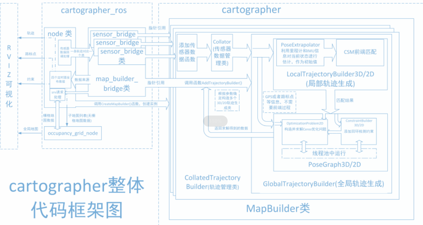
Cartographer uses the mainstream SLAM framework, which is a three-stage structure of feature extraction, closed-loop detection, and back-end optimization. A certain number of LaserScans form a submap, and a series of submaps constitute the global map. The cumulative error in the short-term process of using LaserScan to construct a submap is not large, but the long-term process of using a submap to construct a global map will have a large cumulative error. Therefore, closed-loop detection is needed to correct the positions of these submaps. The basic unit of closed-loop detection is submap, closed-loop detection uses the scan_match strategy. The focus of cartographer is the creation of submap subgraphs that integrate multi-sensor data (odometry, IMU, LaserScan, etc.) and the implementation of the scan_match strategy for closed-loop detection.

• cartographer_ros

cartographer_ros runs under ROS and can accept various sensor data in the form of ROS messages.

After processing, it is published in the form of a message for easy debugging and visualization.

2. Use

2.1. Configuration before use

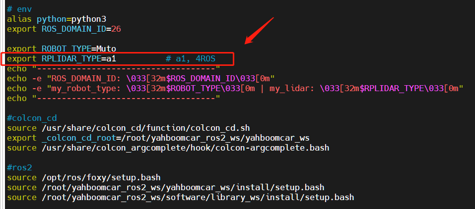
Note: Since the Muto series robots are equipped with multiple lidar devices, the factory system has been configured with routines for multiple devices. However, since the product cannot be automatically recognized, the lidar model needs to be manually set.

After entering the container: Make the following modifications according to the lidar type:

root@ubuntu:/# cd
root@ubuntu:~# vim .bashrc

After the modification is completed, save and exit vim, and then execute:

xxxxxxxxxx
root@jetson-desktop:~# source .bashrc
------------------------------------
ROS_DOMAIN_ID: 26
my_robot_type: Muto | my_lidar: a1
------------------------------------
root@jetson-desktop:~#

You can see the current modified lidar type.

2.2. Specific use

Note: When building a map, the slower the speed, the better the effect (note that the rotation speed should be slower). If the speed is too fast, the effect will be poor.

First, the port binding operation needs to be performed on the host machine [that is, Muto's pi]. The two devices of lidar and serial port are mainly used here;

Then check whether the lidar and serial device are in the port binding state: on the host machine [that is, Muto's pi] refer to the following command to execute the check. The successful binding is as follows:

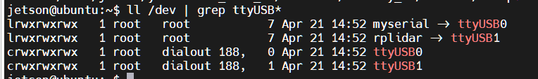
If it shows that the lidar or serial device is not bound, you can plug and unplug the USB cable to check again.

Enter the docker container and execute the following launch file in a terminal:

1. Start mapping

xxxxxxxxxx
ros2 launch yahboomcar_nav map_cartographer_launch.py

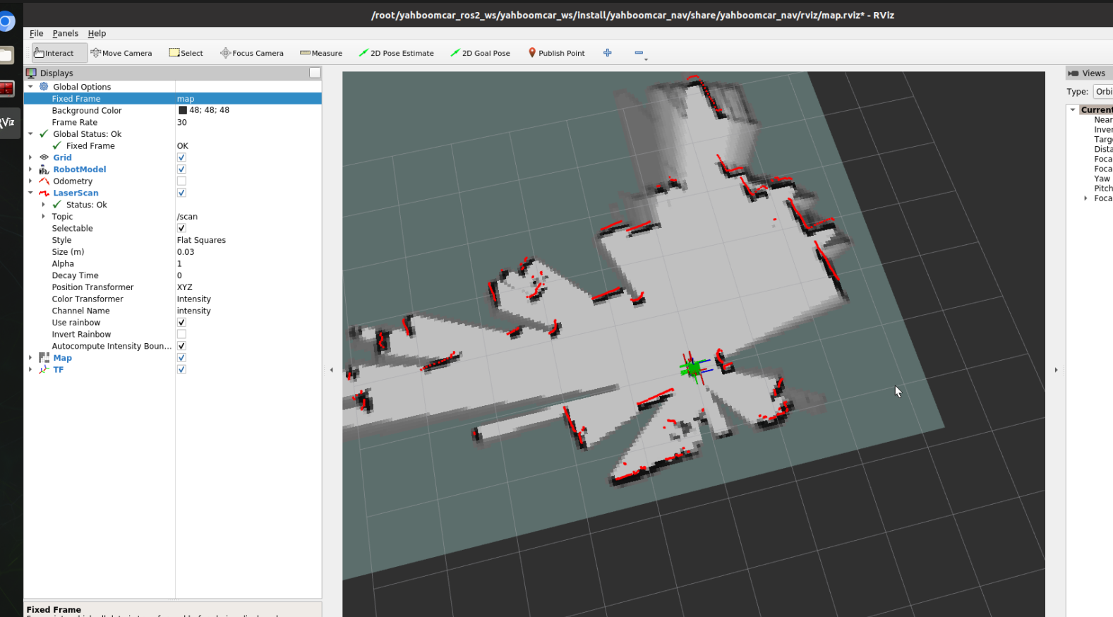
2. Start rviz to display the map. It is recommended to perform this step in a virtual machine. Multi-machine communication needs to be configured in the virtual machine.

xxxxxxxxxx
ros2 launch yahboomcar_nav display_map_launch.py

3. Start the keyboard control node. It is recommended to perform this step in a virtual machine. Multi-machine communication needs to be configured in the virtual machine. Or use the remote control [slowly moving car] to start mapping until a complete map is created

ros2 run yahboomcar_ctrl yahboom_keyboard
# Or
ros2 run teleop_twist_keyboard teleop_twist_keyboard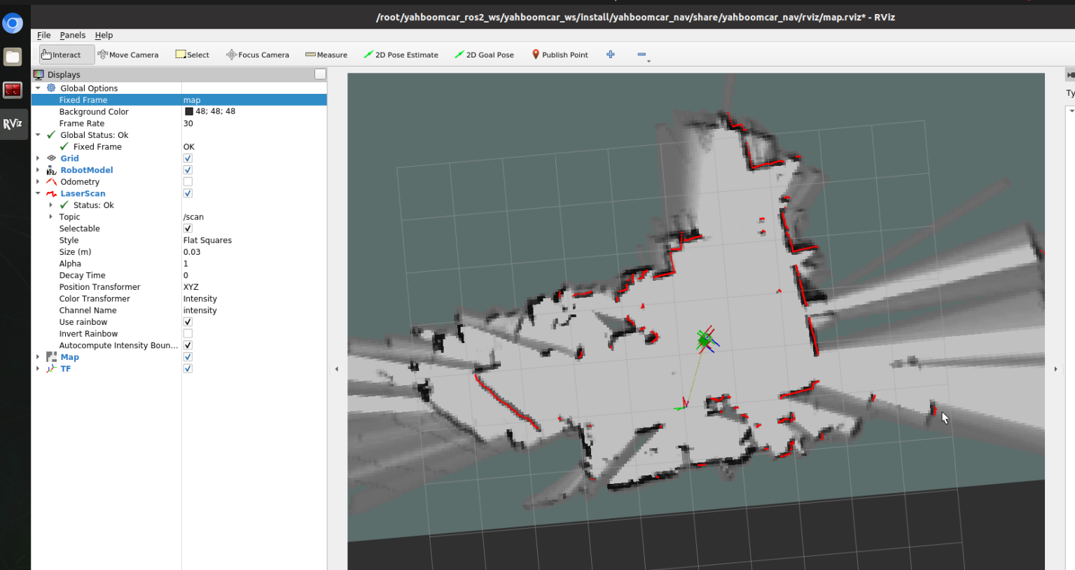

4. Save the map with the following path:

xxxxxxxxxx
ros2 launch yahboomcar_nav save_map_launch.py

Save path is as follows:

xxxxxxxxxx
/root/yahboomcar_ros2_ws/yahboomcar_ws/src/yahboomcar_nav/maps/

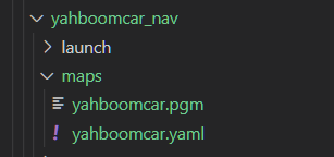
A pgm picture, a yaml file yahboomcar.yaml

xxxxxxxxxx
image: /root/yahboomcar_ros2_ws/yahboomcar_ws/src/yahboomcar_nav/maps/yahboomcar.pgm
mode: trinary
resolution: 0.05
origin: [-10, -10, 0]
negate: 0
occupied_thresh: 0.65
free_thresh: 0.25

Parameter analysis:

• image: The path of the map file, which can be an absolute path or a relative path.
• mode: This attribute can be one of trinary, scale or raw, depending on the selected mode. trinary mode is the default mode
• resolution: resolution of the map, meters/pixel
• Origin: 2D pose (x, y, yaw) in the lower left corner of the map. The yaw here is rotated counterclockwise (yaw=0 means no rotation). Many parts of the current system ignore the yaw value.
• negate: whether to reverse the meaning of white/black and free/occupied (the interpretation of the threshold is not affected)
• occupied_thresh: Pixels with an occupation probability greater than this threshold will be considered fully occupied.
• free_thresh: Pixels with occupancy probability less than this threshold will be considered completely free.

3. Node analysis

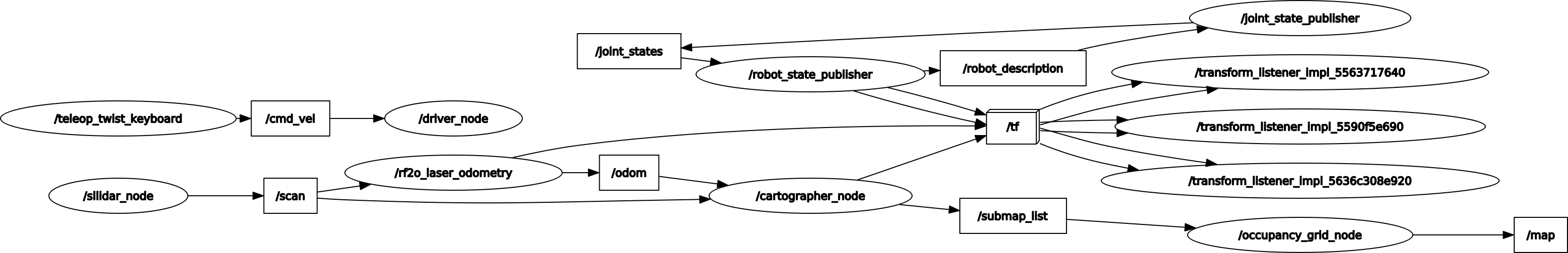
3.1. Display calculation graph

xxxxxxxxxx
rqt_graph

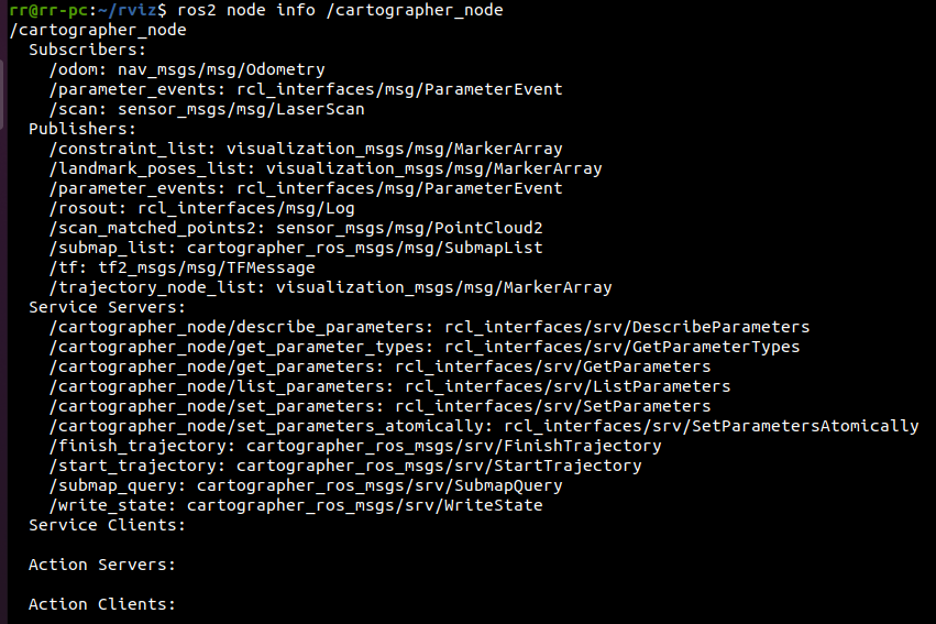
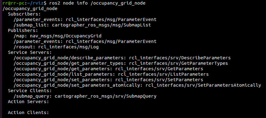
3.2. Cartographer_node node details

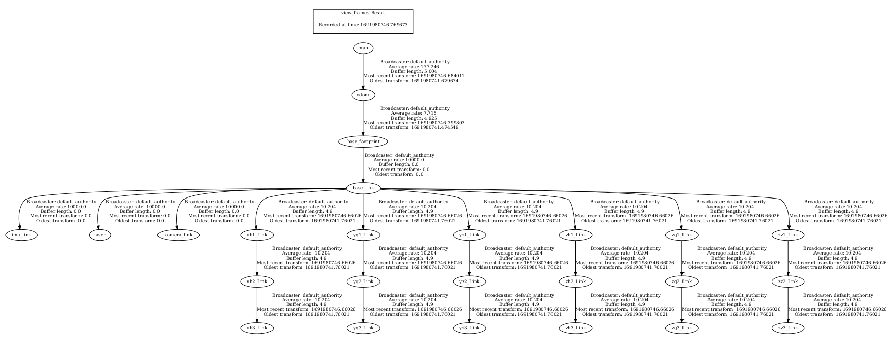
3.3. TF transformation

xxxxxxxxxx
ros2 run tf2_tools view_frames.py