Welcome to AI View Depth camera repository
35.Color tracking
35. Color Tracking
35.1. Introduction
35.1.1. Color Recognition
The color recognition function can recognize multiple colors at any time, store the current recognized color autonomously, and detect the color in real time. It can also realize the function of HSV real-time control. By adjusting the high and low thresholds of HSV, interfering colors are filtered out, so that color blocks can be recognized very ideally in complex environments.
Introduction to HSV
HSV (Hue, Saturation, Value) is a color space created by A. R. Smith in 1978 based on the intuitive characteristics of color, also known as the Hexcone Model.
The color parameters in this model are: hue (H), saturation (S), and brightness (V).
H: 0 — 180
S: 0 — 255
V: 0 — 255
Here, part of the red is classified as the purple range:

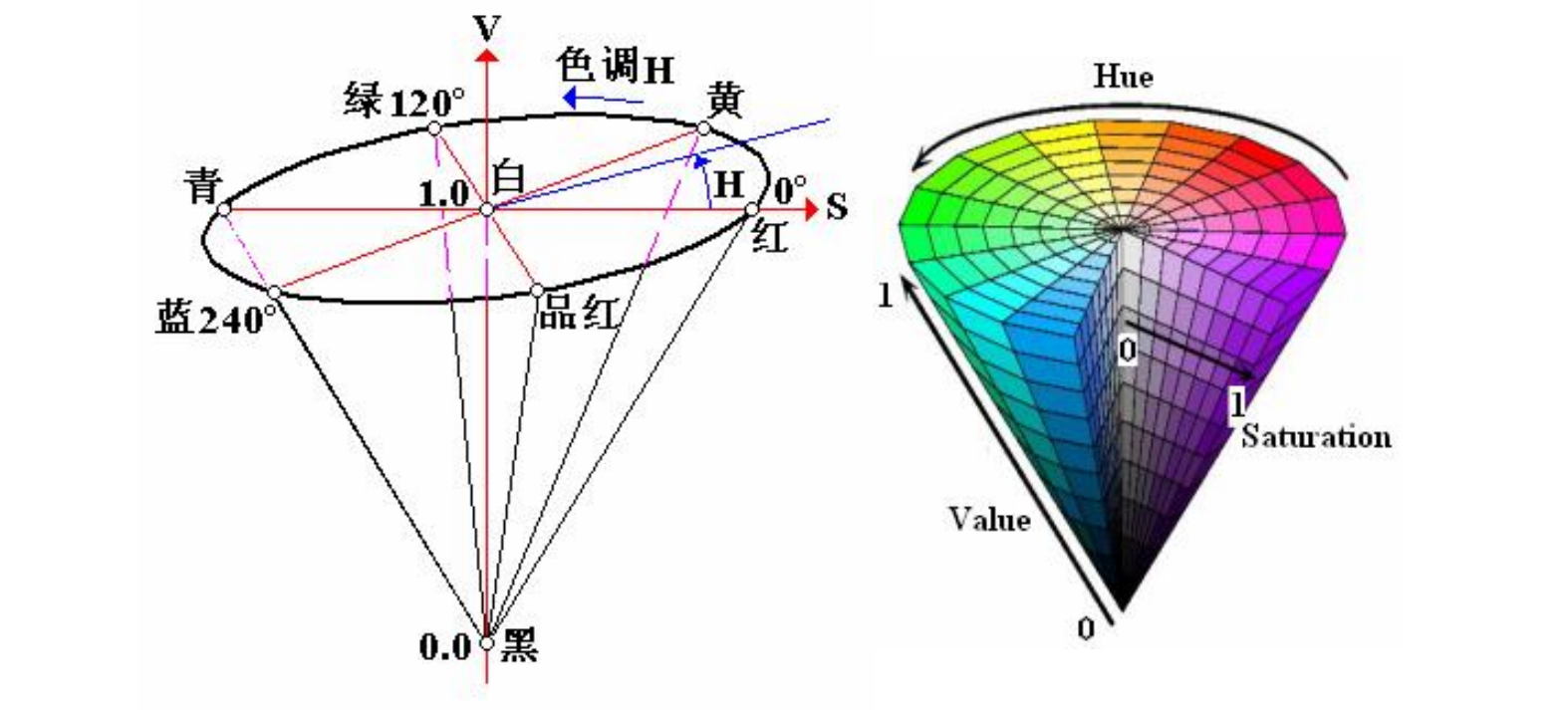
HSV hexagonal pyramid
Hue H
Represents color information, that is, the position of the spectral color. This parameter is expressed as an angle, ranging from 0° to 360°, starting from red and counting counterclockwise, red is 0°, green is 120°, and blue is 240°. Their complementary colors are: yellow is 60°, cyan is 180°, and purple is 300°.
Saturation S
Saturation S is expressed as the ratio between the purity of the selected color and the maximum purity of the color. When S=0, there is only grayscale. 120 degrees apart. Complementary colors differ by 180 degrees. A color can be seen as the result of mixing a certain spectral color with white. The greater the proportion of the spectral color, the closer the color is to the spectral color, and the higher the saturation of the color. The higher the saturation, the deeper and brighter the color. The white light component of the spectral color is 0, and the saturation reaches the highest. The value range is usually 0% to 100%. The larger the value, the more saturated the color.
Brightness V
Brightness indicates the brightness of the color. For the light source color, the brightness value is related to the brightness of the light source; for the object color, this value is related to the transmittance or reflectance of the object. The value range is usually 0% (black) to 100% (white). One thing to note is that there is no direct connection between it and the light intensity.
The three-dimensional representation of the HSV model evolved from the RGB cube. Imagine observing from the white vertex of the RGB along the diagonal of the cube to the black vertex, you can see the hexagonal shape of the cube. The hexagonal boundary represents the color, the horizontal axis represents the purity, and the brightness is measured along the vertical axis.
35.1.2, Brief description of Opencv object tracking algorithm
Object tracking is to locate an object in consecutive video frames. This definition sounds straightforward, but in computer vision and machine learning, tracking is a very broad term that includes conceptually similar but technically different concepts. For example, all the following different but related ideas are usually studied under object tracking:
Dense Optical flow (DOF): These algorithms help estimate the motion vector of each pixel in the video frame.
Sparse optical flow: For example, the Kanade-Lucas-Tomashi (KLT) feature tracking algorithm tracks the position of several feature points in the image.
Kalman Filtering: A very popular signal processing algorithm based on prior motion information, used to predict the position of a moving target. One of the early applications of this algorithm was missile guidance! The onboard computer that guided the Apollo 11 lunar module to the moon had a Kalman filter.
Meanshift and Camshift: These are algorithms for locating the maximum of a density function. They are also used for tracking.
Single object trackers: In this type of tracker, the first frame is marked with a rectangle to indicate the location of the object to be tracked. A tracking algorithm is then used to track the object in subsequent frames. In most real-world applications, these trackers are used in conjunction with an object detector.
Multiple object track finding algorithms: When we have a fast object detector, it makes sense to detect multiple objects in each frame and then run a track finding algorithm to identify which rectangle in one frame corresponds to the rectangle in the next frame.
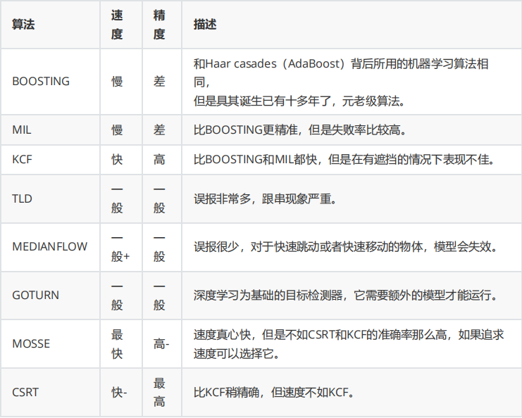
OpenCV Tracking API
35.2, Start
xxxxxxxxxxroslaunch astra_tracker AstraTracker.launch VideoSwitch:=false tracker_type:=colortracker_type parameter: select tracking algorithm ['BOOSTING', 'MIL', 'KCF', 'TLD', 'MEDIANFLOW', 'MOSSE','CSRT', 'color']. You can also switch by pressing the [F] key on the keyboard after startup.
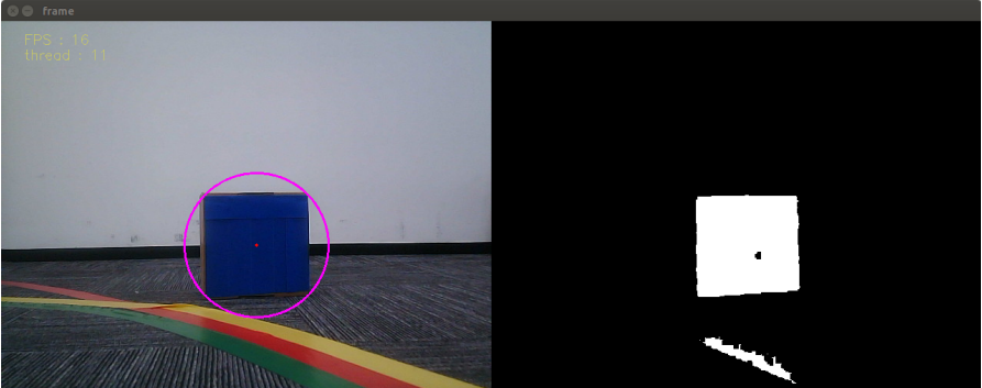
After startup, the system defaults to [Target Detection Mode], as shown below:
[r]: Color selection mode, you can use the mouse to select the area of color to be identified (cannot exceed the area range)
[i]: Target detection mode. Color image on the left, binary image on the right
[f]: Switch algorithm: ['BOOSTING', 'MIL', 'KCF', 'TLD', 'MEDIANFLOW', 'MOSSE', 'CSRT', 'color']
[q]: Exit the program
Color recognition
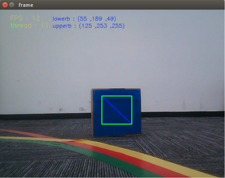
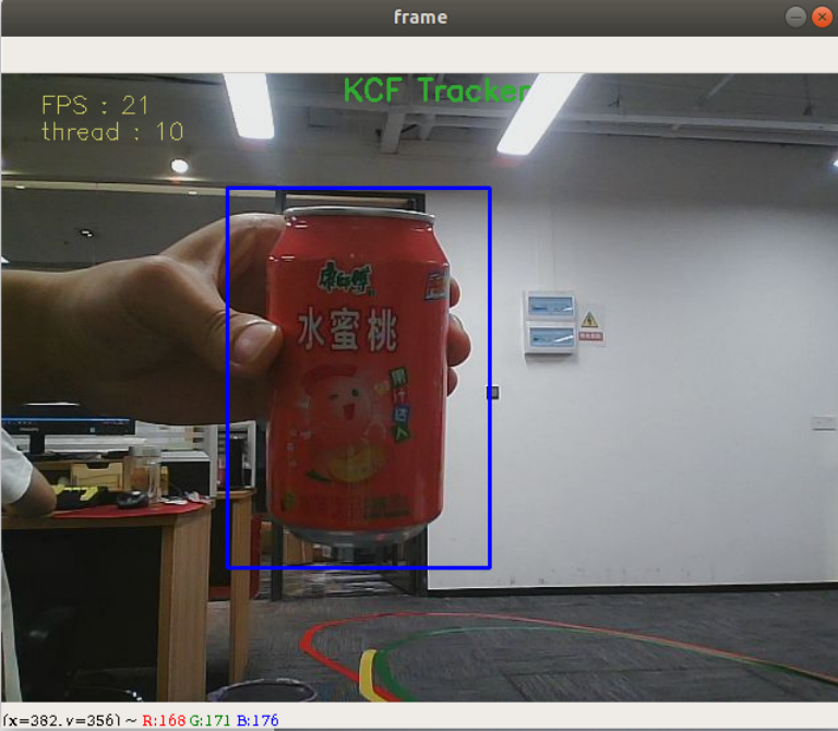
In the color selection mode, use the mouse to select the location of the colored object, as shown in the figure below, and release it to start recognition.
Object tracking
After starting, enter the selection mode, use the mouse to select the location of the object, as shown in the figure below, and release it to start recognition.
35.3, Color Calibration
Dynamic parameter settings,
xxxxxxxxxxrosrun rqt_reconfigure rqt_reconfigure
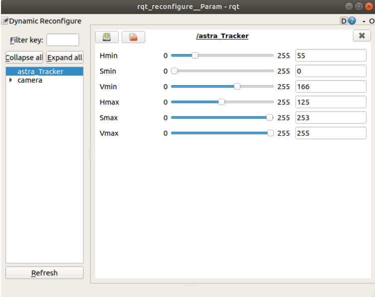
Select the [astra_Tracker] node. Generally, you only need to adjust [Hmin], [Smin], [Vmin], and [Hmax]. These four parameters can be well identified. The slider is always in the dragging state, and the data will not be transferred to the system. It can only be released after it is released; you can also select a row and then slide the mouse wheel.