Welcome to Wheeled Chassis Kit repository

14.3, Kinematic analysis of two-wheel drive car

1. Two-wheel differential kinematic model

The two-wheel differential model refers to the chassis model of the robot chassis consisting of two driving wheels and several supporting wheels.

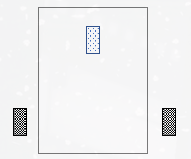
The two-wheel differential model can achieve a certain angular velocity and linear velocity of the robot through different rotation speeds and steering of the two driving wheels.

2. Forward and inverse solution

After understanding the two-wheel differential model, what is the forward and inverse solution?

• Forward kinematics: Forward kinematics focuses on calculating the position and posture of the end effector (such as a manipulator) in space based on the joint parameters of the robot (such as joint angles or displacements). This means that given the configuration of all joints, the position and orientation of the end of the robot can be determined. This calculation usually uses the Denavit-Hartenberg (D-H) parameter method to establish a mathematical model to derive the position and posture of the end effector.
• Inverse kinematics: Inverse kinematics deals with the opposite problem, that is, given the desired position and posture of the end effector, calculate the parameters of each joint required to achieve the posture. This is crucial for path planning and control because it allows determining how the robot needs to move its joints to reach a specific target position. The solution of inverse kinematics is usually more complex than forward kinematics, and there may be multiple solutions or no solutions. Different strategies such as analytical methods, numerical methods or artificial intelligence methods are needed to solve it.

3. Wheel odometer

When we know the relative position between the two wheels and the angular velocity and linear velocity of the robot at each moment, how do we get the current angle and position of the robot?

3.1 Angle

There is only one factor that affects the current angle of the robot, which is the angular velocity.

The angle of the robot's rotation at a certain moment = the angular velocity of the robot at this moment * the duration of this moment

If we assume that the angle of the robot at the initial moment is 0, the current angle of the robot can be obtained by accumulating the angle of the robot's rotation.

The above process is actually to integrate the angular velocity to get the angle.

3.2 Position

By integrating the angular velocity, we get the angle.

The forward speed of the robot in its own direction at a certain moment can be decomposed into the speed in the x-axis and y-axis directions in the odometer coordinate system.

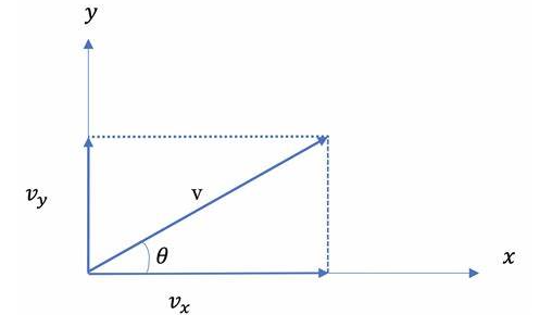
As can be seen from the figure:

vy=v∗cos(θ)

vy=v∗sin(θ)

The speed in the x-axis and y-axis directions is obtained, and the displacement in the x-axis and y-axis directions at this moment can be obtained by multiplying the time corresponding to the speed at a certain moment. The displacement is accumulated to obtain the x and y in the odometer.

4. Derivation of the forward kinematic solution

The two-wheel differential robot is a common type of mobile robot, consisting of two wheels and a center point. We can achieve movement by controlling the rotation speed of each wheel, and can move freely on a plane.

In actual use, we regard the robot as a whole, and for the speed of such a whole in space, we generally use the X-axis velocity v and the Z-axis angular velocity ω to describe it.

It should be noted that in ROS, the front of the robot usually refers to the positive direction of the robot's body coordinate system. The body coordinate system is a coordinate system relative to the robot itself, usually defined at the center of the robot, with the robot's forward direction as the X-axis, the left side as the Y-axis, and the direction perpendicular to the robot plane as the Z-axis**.

The positive direction in the global coordinate system is the X-axis pointing to the right, the Y-axis pointing forward, and the Z-axis perpendicular to the ground**.

	X	Y	Z
Robot body coordinate system	Front	Left	Perpendicular to the robot plane
Global coordinate system	Right	Front	Perpendicular to the ground

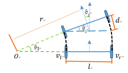
So the problem becomes assuming that the robot's left and right wheel linear velocities vl and vr remain constant for a short period of time t, and the installation spacing between the two wheels is l, and find the robot's linear velocity v and angular velocity ω.

Let's look at the above figure to deduce that because the robot's linear velocity direction and the wheel rotation direction are always consistent, the robot's linear velocity is the average of the right wheel linear velocity, that is:

v=(vl+vr)/2

We know:

v=ω∗r

According to the above figure, we have:

l=rr−rl

=vr/ωr−vl/ωl

The same robot has the same angular velocity, so we have:

ωl=ωr

We can find:

ω=(vr−vl)/l