Balance car mathematical model

Classic inverted pendulum mathematical model

The inverted pendulum system usually consists of a rotatable rod and a mass block, the mass block is located at one end of the rod, and the entire system is controlled by a motor or other driver.

xxxxxxxxxx
The goal of controlling the inverted pendulum system is to keep the mass block in a vertical position and be robust to external interference

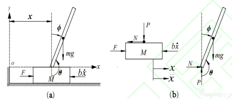
Figure (a) is a simplified model diagram of the inverted pendulum system, and Figure (b) is a force analysis diagram of the inverted pendulum system

Instructions

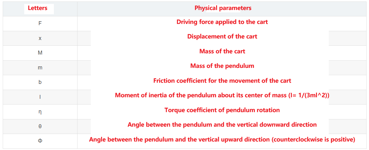
Based on Newton's mechanics and theorem of motion, the process of deriving the dynamic equation of the linear inverted pendulum system is as follows: Analyze the force balance of the car in the horizontal direction

Analyze the force balance of the pendulum in the horizontal direction, and we can get:

(1) and (2) In the equations, N is the interaction force between the slider and the pendulum in the horizontal direction. Combining the two equations (1) and (2) eliminates N, we get the first nonlinear dynamics model equation of the first-order linear inverted pendulum:

Analyzing the force balance of the pendulum in the vertical direction, we get:

Analyzing the moment balance of the pendulum around its center of mass, we get:

In equations (2), (4), and (5), N and P are the interaction forces between the slider and the pendulum in the horizontal and vertical directions. Combining equations (2), (4), and (5) eliminates P, N, we get the second nonlinear dynamic model equation of the first-order linear inverted pendulum:

The inverted pendulum is stable when -0.3rad < Φ <0.3rad, and the swing angle Φ is very small, so:

Therefore, the nonlinear dynamic equation (3) of the inverted pendulum system can be Linearize with (6) to obtain the linearized dynamic equation of the first-order linear inverted pendulum system:

Remember the state vector:

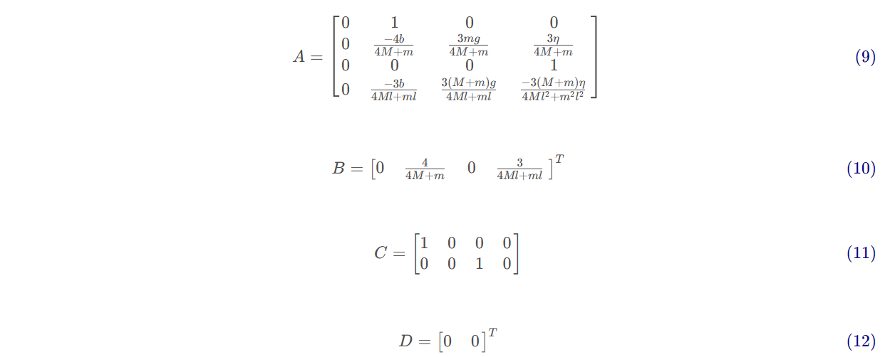
With u=F, according to equation group (7) The state space equation of the first-order linear inverted pendulum system is as follows:

Balance car mathematical model

The balance car is a small car that achieves self-balancing through two wheels. Its structure mainly consists of a car body and two wheels. The mathematical model can be regarded as a moving inverted pendulum.

xxxxxxxxxx
The MPU6050 detects its posture information, and after processing by the processor, it will control the robot's motor so that the robot can reach a stable state.

Wheel model

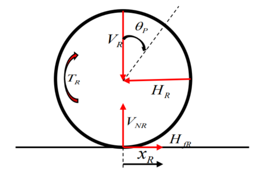
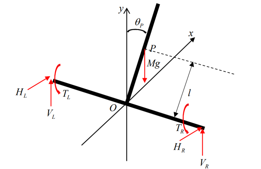
The force analysis diagram of the left and right wheels of the two-wheeled robot is shown in the figure. The horizontal force of the robot is the vector sum of the friction between the wheel and the ground and the horizontal force between the body and the wheel.

The movement of the balancing car is achieved by the rotation of the wheels. We choose a pair of coaxially installed wheels with the same parameters (mass, moment of inertia, radius).

Take the right wheel as an example for force analysis:

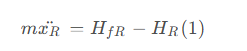
The movement of the wheel can be decomposed into translation and rotation, and Newton's second law can be obtained:

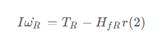
From the law of rigid body fixed axis rotation, it can be obtained:

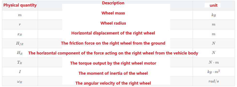
Explanation

Combining (1) and (2), we get:

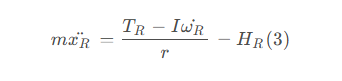
When the wheel does not slip, the speed of the wheel is proportional to the speed of rotation, that is,

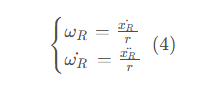
Combining (3) and (4), we get:

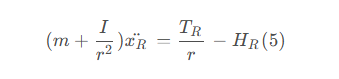
Since the parameters of the left and right wheels are the same, the left wheel has a similar result, that is,

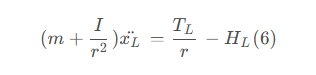
Car body model

The movement of the car body can also be decomposed into forward movement (forward, pitch) and lateral movement (steering, yaw): yaw movement can be regarded as a special case of steering movement.

Forward motion

The forward motion of the car can be decomposed into forward motion and relative rotation (pitch) around the center of mass P of the car body:

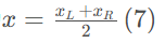
The horizontal displacement of the center O of the chassis of the car is:

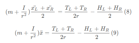
Add equations (5) and (6) together, and divide both sides of the equation by 2 to get:

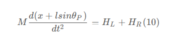
Apply Newton's second law to the car body, in the horizontal direction:

Apply Newton's second law to the car body, in the vertical direction:

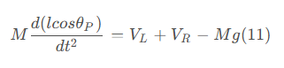
Apply the law of rigid body fixed axis rotation to the car body and we get:

Explanation

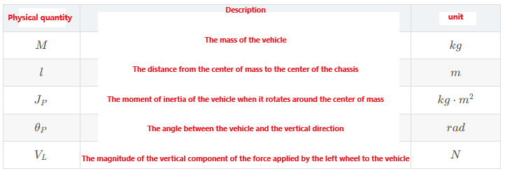
The combined equations (9) and (10) yield:

Among them:

The equation contains nonlinear terms, so it is linearized. Considering that the inclination angle of the vehicle body is relatively small, it can be considered that:

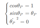
Therefore, equation (13):

Substitute equations (10) and (11) into equation (12):

Linearize equation (15):

Substitute equation (16) into equation (14):

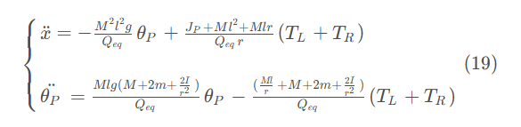
In summary, for forward motion:

Steering movement

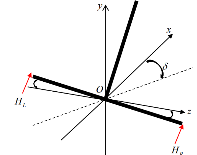
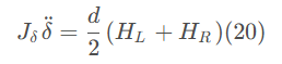
The steering movement is caused by the unequal magnitudes of the reaction forces HL and HR applied to the vehicle body by the left and right wheels in the horizontal direction. According to the law of rigid body fixed axis rotation, we can get:

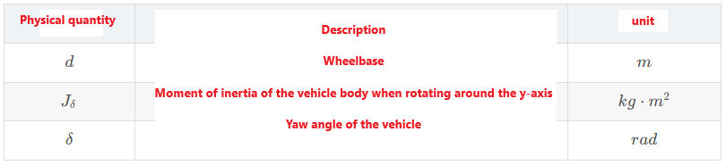
Explanation

Subtract equations (5) and (6) to get:

When the left and right wheels have different speeds, the vehicle body turns:

According to the geometric relationship, we can get:

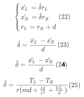
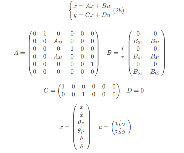
From equations (19) and (25), we can get the state equation of the system:

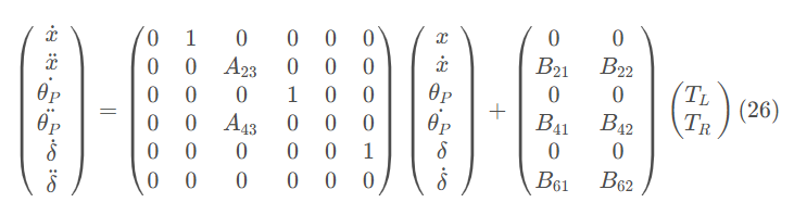
The state variables represent the displacement, forward speed, inclination angle, angular velocity, steering angle and steering speed of the car.

Since the magnitude of the motor output torque is difficult to control directly, it is converted into the acceleration of the two wheels through the law of rigid body fixed axis rotation:

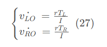
The left side of equation (27) is the magnitude of the linear velocity of the left/right wheel when there is no friction (in rad/s).

Therefore, the state space expression of the system becomes: