Welcome to ROSMASTER R2 repository

1、PID algorithm theory

1.1、Introduction to algorithms

PID is to perform proportional integral differentiation on the input deviation, and the superposition results of the operation are used to control the actuator. The formula is as follows :

$u(t)=K_p[e(t)+frac{1}{T_i}int_{0}^{t}e(t)dt+Tdfrac{de(t)}{dt}]$

It consists of three parts:

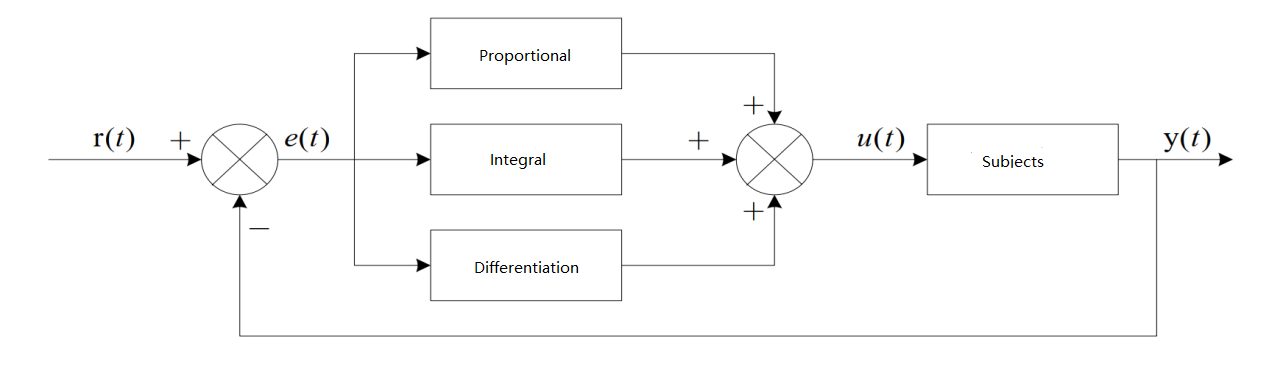
• P is the proportion, which is the input deviation multiplied by a coefficient;

• I is the integral, which is the integral operation of the input deviation;

• D is differentiation, which differentiates the input deviation.

The following figure shows a basic PID controller:

1.1.1、proportional part

The mathematical representation of the proportional part is: $K_p*e(t)$

In analog PID controllers, the proportional link reacts instantaneously to deviations. Once the deviation occurs, the controller immediately produces a control effect, so that the control quantity changes in the direction of reducing the deviation. The strength of the control effect depends on the scale coefficient, the larger the scale coefficient, the stronger the control effect, the faster the transition process, the smaller the static deviation of the control process; However, the larger it is, the easier it is to oscillate and destabilize the system. Therefore, the example coefficient selection must be appropriate to achieve a small transition time and a small static difference and stable effect.

Advantages: Adjust the open-loop scale coefficient of the system, improve the steady-state accuracy of the system, reduce the inertia of the system, and speed up the response speed.

Disadvantages: With only the P controller, the excessive open-loop scale coefficient will not only increase the overshoot of the system, but also make the system stability margin smaller or even unstable.

1.1.2、Points section

The mathematical representation of the integral part is: $frac{K_p}{T_i}int_{0}^{t}e(t)dt$ The larger the integral constant, the weaker the accumulation of integrals, and the system will not oscillate during the transition; However, increasing the integration constant will slow down the elimination process of static error, and the time required to eliminate the deviation is longer, but it can reduce the overshoot and improve the stability of the system. When Ti is small, the integration effect is stronger, and oscillations may occur in the system transition time, but the time required to eliminate the deviation is shorter. Therefore, Ti must be determined according to the specific requirements of actual control.

Advantages: Eliminates steady-state errors.

Disadvantages: The addition of the integral controller will affect the stability of the system and reduce the stability margin of the system.

1.1.3、differential part

The mathematical representation of the differential part is: $K_p*Tdfrac{de(t)}{dt}$

The role of the differential link makes the deviation stop. It is controlled according to the trend of change of deviation (speed of change). The faster the deviation changes, the larger the output of the differential controller and can be corrected before the deviation value becomes larger. The introduction of differential action will help to reduce the overshoot, overcome oscillation, and stabilize the system, especially for the order system, which is very beneficial to the tracking speed of the system. However, the role of differentiation is sensitive to the noise of the input signal, and those noisy systems generally do not use differentiation, or filter the input signal before the differentiation works. The role of the differential part is determined by the differential time constant Td. The larger the Td, the stronger its effect on suppressing deviation changes; The smaller the Td, the weaker it is to resist changes in deviation. The differential part obviously has a great effect on system stability. Proper selection of the differential constant Td can optimize the differential action.

Advantages: make the response speed of the system faster, overshoot is reduced, oscillation is reduced, and has a "prediction" effect on the dynamic process.

1.2、selection of PID algorithm

Digital PID control algorithms can be divided into positional PID and incremental PID control algorithms. So before we decide which PID algorithm to use, we should first understand his principle:

1.2.1、positional PID algorithm

$u(k)=K_pe(k)+K_Isum_{i=o}e(i)+K_D[e(k)-e(k-1)]$

e(k): User-set value (target value) - The current state value of the control object

Scale P : e(k)

Integral I: ∑ accumulation of e(i) errors

Differential D : e(k) - e(k-1) This error - last error

That is, the positional PID is the actual position of the current system, and the deviation from the expected position you want to achieve is controlled by PID

Because there is an error integral ∑e(i), which is always accumulated, that is, the current output u(k) is related to all past states, the cumulative value of the error is used; (error e will have error accumulation), the output u(k) corresponds to the actual position of the actuator, once the control output is wrong (the current state value of the control object is a problem), a large change in u(k) will cause a large change in the system and positional PID when the integral term reaches saturation, the error will still continue to accumulate under the action of integration, once the error begins to change in reverse, the system needs a certain time to exit from the saturation region, so in u(k) reaches the maximum and minimum, to stop the integration action, And there must be integral limiting and output limiting, so when using positional PID, we generally use PD control directly

Positional PIDs, on the other hand, are suitable for the control of upright and temperature control systems for actuators without integral parts, such as servos and balance trolleys

Advantages: Positional PID is a non-recursive algorithm that directly controls the actuator (such as the balance trolley), and the value of u(k) and the actual position of the actuator (such as the current angle of the trolley) correspond one-to-one, so it can be well applied in objects without integral parts of the actuator

Disadvantages: Each output is related to the past state, and e(k) is accumulated when calculating, which is a large amount of computational work.

1.2.2、incremental PID algorithm

$Delta u(k)=u(k)-u(k-1)=K_P[e(k)-e(k-1)]+K_ie(k)+K_D[e(k)-2e(k-1)+e(k-2)]$

Scale P : $e(k)-e(k-1)$ this time error - last error

Integral I: $e(k)$ error

Differential D : $e(k)-2e(k-1)+e(k-2)$ this time error -2 * last error + last error

Incremental PID can be well seen according to the formula, once the KP, TI, TD, as long as the deviation of the three measurements before and after is used, the control amount $Delta u(k)$ obtained by the formula can be found by the formula The control amount $Delta u(k)$ corresponds to the increment of the recent position error, rather than corresponding to the deviation from the actual position There is no error accumulation, that is, there is no need to accumulate in incremental PID. The determination of the control increment $Delta u(k)$ is only related to the last 3 sampling values, which is easy to obtain a better control effect through weighting processing, and when problems occur in the system, incremental will not seriously affect the work of the system

Summary: Incremental PID is an increment of positional PID, at which time the controller outputs the difference between the position values calculated at the adjacent two sampling moments, and the result is the increment, that is, the control quantity needs to be increased (negative value means reduce) on the basis of the previous control quantity.

Merit:

(1) The impact is small when the operation is small, and the error data can be removed by logical judgment if necessary.

(2) The impact is small during manual/automatic switching, which is convenient to achieve no disturbance switching. When the computer fails, it remains the same.

(3) There is no need to accumulate in the calculation. The determination of the control increment Δu(k) is only relevant to the last 3 sampling values.

Shortcoming:

(1) The integral truncation effect is large and there is a steady-state error;

(2) The impact of spillage is large. Some subjects are not very good with incremental type;

1.2.3、The difference between incremental and positional

1.2.3、Difference between incremental and positional

(1) The incremental algorithm does not need to be accumulated, and the determination of the increment of the control quantity is only related to the recent deviation sampling value, and the calculation error has little impact on the control quantity calculation. The positional algorithm uses the accumulation value of the past deviation, which is easy to produce a large accumulation error.

(2) The incremental algorithm obtains the increment of the control quantity, for example, in the valve control, only the change part of the valve opening is output, the impact of misoperation is small, and if necessary, the output can be limited or prohibited by logical judgment, which will not seriously affect the work of the system. The output of the positional type directly corresponds to the output of the object, so it has a greater impact on the system.

(3) The incremental PID control output is the increment of the control amount and has no integration effect, so the method is suitable for the object of the actuator with integral parts, such as stepper motors, etc., while the positional PID is suitable for the object without integral parts of the actuator, such as electro-hydraulic servo valves.

(4) When performing PID control, positional PID needs to have integral limiting and output limiting, while incremental PID only needs output limiting

Positional PID and incremental PID are just two implementations of digital PID control algorithms, which are essentially identical. The main difference is that the integration items are stored in different ways, positional PID points are stored separately, incremental PID points are stored as part of the output, and online players also have their own unique insights and views on the use of positional and incremental, depending on which algorithm is suitable for our specific application scenarios.

1.3、debugging of PID parameters

There are many methods for selecting PID controller parameters, such as trial method, critical proportionality method, extended critical proportionality method, etc. However, for PID control, the selection of parameters is always a very troublesome work, and it needs to be constantly adjusted to obtain a more satisfactory control effect. Based on experience, the steps for determining general PID parameters are as follows:

1.3.1、determine the scale factor Kp

When determining the scale coefficient Kp, first remove the integral term and differential term of PID, so that Ti=0 and Td=0 make it a pure proportional adjustment. The input is set to 60%~70% of the maximum allowable output of the system, and the scale coefficient Kp gradually increases from 0 until the system oscillates; In turn, the scale factor Kp gradually decreases from this time until the system oscillation disappears. Record the scale factor Kp at this time, and set the scale factor Kp of PID to 60%~70% of the current value.

1.3.2、Determine the integration time constant Ti

After the scale factor Kp is determined, set a large integration time constant Ti, then gradually decrease Ti until the system oscillates, and then conversely, gradually increase Ti until the system oscillations disappear. Record Ti at this time, and set the integration time constant Ti of PID to 150%~180% of the current value.

1.3.3、Determine the differential time constant Td

The differential time constant Td generally does not need to be set, it can be 0, and the PID adjustment is converted to PI adjustment. If it needs to be set, it is determined in the same way as Kp, taking 30% of its value when it is not oscillating.

1.3.4、system no-load, on-load joint debugging

Fine-tune PID parameters until performance requirements are met.

Of course, this is just my personal debugging method, not necessarily suitable for everyone and every environment, only for your reference; However, there are also classic tips for debugging PID circulating on the Internet.

PID is a proportional (P), integral (I), differential (D) control algorithm, not necessarily have to have these three algorithms at the same time, can also be PD, PI, or even only P algorithm control. One of my simplest ideas for closed-loop control before is only P control, feedback the current result back, and then subtract from the target, if it is positive, it will slow down, if it is negative, it will accelerate, of course, this is only the simplest closed-loop control algorithm, and it is still back to the previous section of positional and incremental summary, specifically refer to our current control environment, because of the difference in each control system, the parameters that can make our system achieve the most stable effect are OK.