Welcome to Transbot SE repository
3.Basic use of PyTorch(jetson)
3 Basic use of PyTorch
3 Basic use of PyTorch 3.1 About PyTorch 3.1.1 Introduction 3.1.2 Features 3.2 Tensors in PyTorch 3.2.1 Tensor 3.2.2 create a tensor 3.3 torchvision package introduction 3.3.1 torchvision is a library dedicated to processing images in Pytorch, including four categories: 3.4 Convolutional Neural Networks 3.4.1 Neural network 3.4.2 Convolutional Neural Networks 3.5 Build the LetNet neural network and train the data set 3.5.1 Preparation before implementation 3.5.2 Implementation process 3.5.3 Running the program

The Raspberry Pi motherboard series does not support the PyTorch function yet.
3.1 About PyTorch
3.1.1 Introduction
PyTorch is an source open Python machine learning library, based on Torch, for applications such as natural language processing.
3.1.2 Features
- powerful GPU-accelerated tensor computing
- deep neural network of automatic derivation system
- dynamic graph mechanism
3.2 Tensors in PyTorch
3.2.1 Tensor
The English of tensor is Tensor, which is the basic operation unit in PyTorch. Like Numpy's ndarray, it represents a multi-dimensional matrix. The biggest difference from ndarray is that PyTorch's Tensor can run on GPU, while numpy's ndarray can only run on CPU, and running on GPU greatly speeds up the operation.
3.2.2 create a tensor
- There are many ways to create tensors. Calling APIs of different interfaces can create different types of tensors.
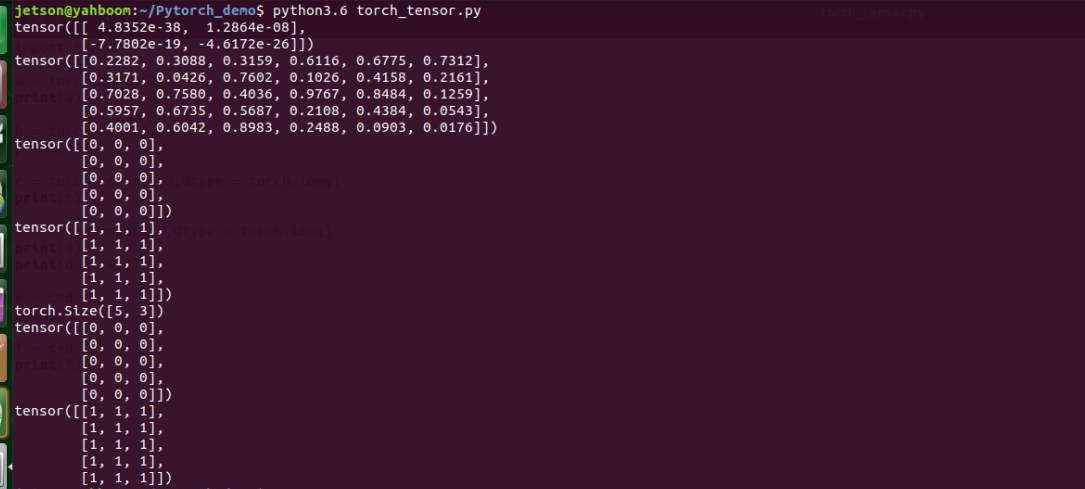
a = torch.empty(2,2): create an uninitialized 2*2 tensor
b = torch.rand(5, 6) : creates a uniformly distributed initialization tensor with each element from 0-1
c = torch.zeros(5, 5, dtype=torch.long): Create an initialized all-zero tensor and specify the type of each element as long
d = c.new_ones(5, 3, dtype=torch.double) : create a new tensor d based on a known tensor c
d.size(): Get the shape of the tensor d
- Operations between tensors
The operation between tensors is actually the operation between matrices. Due to the dynamic graph mechanism, mathematical calculations can be performed directly on the tensors. For example,
Add two tensors:
c = torch.zeros(5,3,dtype=torch.long)d = torch.ones(5,3,dtype=torch.long)e = c + dprint(e)Multiply two tensors
xxxxxxxxxxc = torch.zeros(5,3,dtype=torch.long)d = torch.ones(5,3,dtype=torch.long)e = c * dprint(e)
This part of the code can be referred to: ~/Pytorch_demo/torch_tensor.py
run the code,
xxxxxxxxxxpython3 torch_tensor.py
3.3 torchvision package introduction
3.3.1 torchvision is a library dedicated to processing images in Pytorch, including four categories:
- torchvision.datasets: load datasets, Pytorch has many datasets such as CIFAR, MNIST, etc., you can use this class to load datasets, the usage is as follows:
xxxxxxxxxxcifar_train_data = torchvision.datasets.CIFAR10(root = './data', train = True, download = False, transform = transform) - torchvision.models: Load the trained model, the model includes the following VCG, ResNet, etc. The usage is as follows:
xxxxxxxxxximport torchvision.models as models resnet18 = models.resnet18() - torchvision.transforms: the class of image transformation operation, the usage is as follows:
xxxxxxxxxxtransform = transforms.Compose( [ transforms.ToTensor(), transforms.Normalize((0.5, 0.5, 0.5),(0.5, 0.5, 0.5))]) - torchvision.untils: Arrange the pictures into a grid shape, the usage is as follows:
xxxxxxxxxxtorchvision.utils.make_grid(tensor, nrow = 8, padding = 2, normalize = False, range = None, scale_each = False, pad_value = 0) For more information on the use of the torchvision package, you can refer to the official website documentation: https://pytorch.org/vision/0.8/datasets.html
3.4 Convolutional Neural Networks
3.4.1 Neural network
- The difference between neural network and machine learning
Both neural networks and machine learning are used for classification tasks. The difference is that neural networks are more efficient than machine learning, the data is simpler, and fewer parameters are required to perform tasks. The following points are explained:
- Efficiency: The efficiency of neural networks is reflected in the extraction of features. It is different from the features of machine learning. It can be trained and "corrected" by itself. We only need to input data, and it will continuously update the features by itself.
- Data simplicity: In the process of machine learning, we need to perform some processing on the data before inputting the data, such as normalization, format conversion, etc., but in the neural network, it does not require too much processing.
- Fewer parameters to perform tasks: In machine learning, we need to adjust penalty factors, slack variables, etc. to tune to the most suitable effect, but for neural networks, only a weight w and bias term b need to be given, During the training process, these two values will be continuously revised and adjusted to the optimum, so that the error of the model is minimized.
3.4.2 Convolutional Neural Networks
- convolution kernel
Convolution kernels can be understood as feature extractors, filters(digital signal processing), and so on. The neural network has three layers(input layer, hidden layer, output layer), and the neurons in each layer can share the convolution kernel, so it is very convenient to process high-level data. We only need to design the size, number and sliding step size of the convolution kernel to make it train by itself.
- the three basic layers of the convolutional neural network:
convolutional layer
Perform convolution operation, inner product operation of two convolution kernel-sized matrices, multiply the numbers in the same position and then add and sum. A small number of convolution kernels are set in the convolutional layer close to the input layer, and the further the convolutional layer is, the more convolutional kernels are set in the convolutional layer.
pooling layer
By downsampling, the image and parameters are compressed, but the quality of the image is not destroyed. There are two pooling methods, MaxPooling(that is, taking the largest value in the sliding window) and AveragePooling(taking the average of all the values in the sliding window).
Flatten layer & Fully Connected layer
This layer is mainly a stack of layers. After the pooling layer, the image is compressed, and then goes to the Flatten layer; the output of the Flatten layer is put into the Fully Connected layer, and softmax is used to classify it.
3.5 Build the LetNet neural network and train the data set
3.5.1 Preparation before implementation
- the environment
The ROSMASTER-jetson development board series are all installed with the project development environment, including:
- python 3.6+
- torch 1.8.0
- torchvision 0.9.0
- data set
CIFAR-10, 50,000 training images of 32*32 size, and 10,000 test images
Note: The dataset is saved in the ~/Pytorch_demo/data/cifar-10-batches-py directory,
| Filename | file usage |
|---|---|
| batches.meta.bet | The file stores the English name of each category. It can be opened and viewed with Notepad or other text file readers |
| data batch 1.bin | These 5 files are training data in the CIFAR-10 dataset. Each file stores 10,000 32 x 32 color images and their corresponding class labels in binary format. |
| data batch 2.bin | . |
| data batch 3.bin | . |
| data batch 4.bin | . |
| data batch 5.bin | A total of 50,000 training images |
| test batch bin | This file stores the test images and the labels of the test images. A total of 10,000 sheets |
| readme. html | Dataset introduction file |
| Tensor type | describe |
|---|---|
| tf.float32 | 32-bit floating point number |
| tf.float64 | 64-bit floating point |
| tf.int64 | 64-bit signed integer |
| tf.int32 | 32-bit signed integer |
| tf.int16 | 16-bit signed integer |
| tf.int8 | 8-bit signed integer |
| tf.uint8 | 8-bit unsigned integer |
| tf.string | variable length byte array |
| tf.bool | boolean |
| tf.complex64 | real and imaginary numbers |
3.5.2 Implementation process
- import related modules
xxxxxxxxxximport torch import torch.nn as nn import torch.nn.functional as F import torchvision import torchvision.transforms as transforms import torch.optim as optim - load the dataset
xxxxxxxxxxcifar_train_data = torchvision.datasets.CIFAR10(root = './data', train = True, download = False, transform = transform) cifar_test_data = torchvision.datasets.CIFAR10(root = './data', train = False, transform = transform) - package data set
xxxxxxxxxxtrain_data_loader = torch.utils.data.DataLoader(cifar_train_data, batch_size = 32, shuffle = True) test_data_loader = torch.utils.data.DataLoader(cifar_test_data, batch_size = 32, shuffle = True - build a convolutional neural network
xxxxxxxxxxclass LeNet(nn.Module): #Define the operation operators required by the network, such as convolution, fully connected operators, etc. def __init__(self): super(LeNet, self). __init__() #Conv2d parameter meaning: number of input channels, number of output channels, kernel size self.conv1 = nn.Conv2d(3, 6, 5) self.conv2 = nn.Conv2d(6, 16, 5) self.fc1 = nn.Linear(16 * 5 * 5, 120) self.fc2 = nn.Linear(120, 84) self.fc3 = nn.Linear(84, 10) self.pool = nn.MaxPool2d(2, 2) def forward(self, x): x = F.relu(self.conv1(x)) x = self.pool(x) x = F.relu(self.conv2(x)) x = self.pool(x) x = x.view(- 1, 16 * 5 * 5) x = F.relu(self.fc1(x)) x = F.relu(self.fc2(x)) x = self.fc3(x) return x - configure the loss function and optimizer for training
xxxxxxxxxxcriterion = nn.CrossEntropyLoss() optimizer = optim.SGD(net.parameters(), lr = 0.005, momentum = 0.9) - start training and testing
3.5.3 Running the program
- reference code path
xxxxxxxxxx~/Pytorch_demo/pytorch_demo.py - run the program
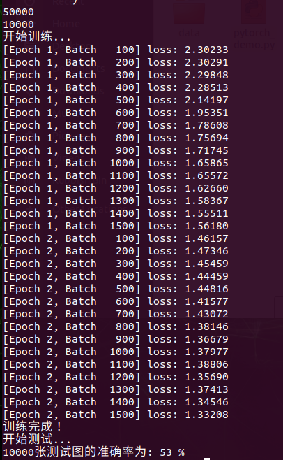
xxxxxxxxxxcd ~/Pytorch_demo python3 pytorch_demo.py xxxxxxxxxxcd ~/Pytorch_demopython3 pytorch_demo.py
 |  |
|---|
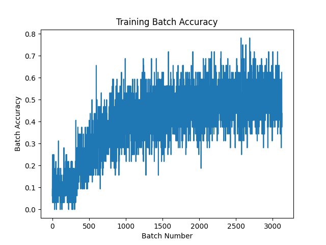
We have only trained 2 times here. You can modify the eTOCh value to modify the training times. The more training times, the higher the accuracy.